Poisson distribution and the family of its related distributions (part I)

Mohamadreza Fazel

July 2023

In our daily life, we encounter many incidences with binary outcomes, such as passing or failing a test, a rainy or sunny afternoon, winning a lottery or not, and many more. The aim of this post is to approach such binary events from a mathematical point of view. In this context, a probability is assigned to each outcome and the outcome is described by a Binomial distribution. Here, we begin by describing the Binomial distribution and proceed to derive Poisson distribution as its limit. We next illustrate a few other distributions related to Poisson such as Exponential distribution in part I, and relegate Erlang distribution, Gamma distribution and Normal distribution to part II of this post. These distributions are related to the Poisson distribution in one of the following ways: they 1) are limits of Poisson distribution; 2) describe the waiting times between Poisson events.

Binomial Distribution

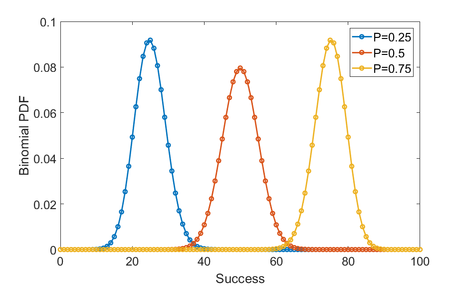
To describe the Binomial distribution, we begin by illustrating the Bernoulli trial. A Bernoulli trial is a process with only two possible outcomes. For instance, flipping a coin is a Bernoulli trial since the outcome is either a head or a tail. Another example is the success or failure of an experiment or an attempt to achieve a goal. If one conducts multiple Bernoulli experiments, the number of successes k would be a number between zero and the number of experiments and is termed a Binomial random variable following the distribution $${\mathrm{Binomial}(k;n,p)=\frac{n!}{k!(n-k)!}p^k(1-p)^{(n-k)}}\tag{1}$$ where n and p are, respectively, the number of Bernoulli trials (experiments) and the probability of success in a trial. A few examples of Bernoulli distributions are shown in Fig. 1.

Poisson Distribution

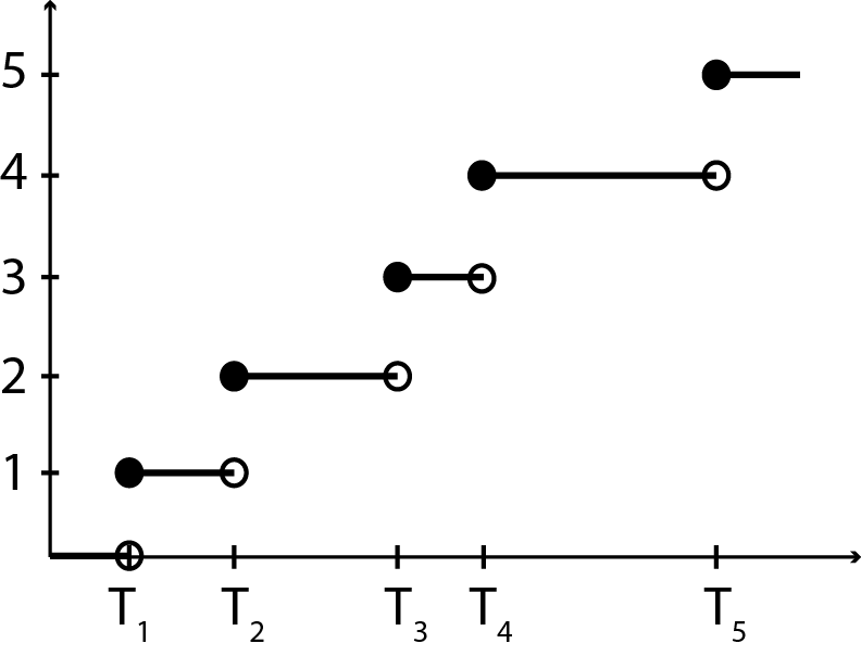
Now, we show that the Poisson distribution is a limit of Binomial distribution when the success probability is small. To do so, we start by describing the counting process. A counting process is a random process that enumerates the number of times an incident (success) has occurred from the beginning up to a time t,  {N_t, t ≥ 0}, where N_t is the number of events up to the time t. A sample path of such a process is shown in Fig. 2. For two given times 0 ≤ t₁ < t₂, we have N_t1 ≤ N_t2, and the number of events that has happened between times t₁ and t₂ is thus k = N_t2 − N_t1. k is called increment of the process.

Now, we introduce the Poisson process. A counting process is called a Poisson process if:

1. The probability of having more than one event in a short time interval is essentially zero.
2. The probability of a random event in a short time interval is only proportional to the length of the time interval and not where the time interval is located with respect to the origin (t = 0).
3. The numbers of random events occurring in non-overlapping time intervals are independent.

Using these axioms, we can derive the Poisson distribution. According to the first axiom, in a short time interval, Δt, an event can either occur or not occur, which is a Bernoulli trial. If the rate of event occurrence is given by λ, then by the second axiom the probability of an event taking place over the time interval Δt is p = λΔt. Now, considering n attempts (Bernoulli trials) over a time interval T = nΔt, what is the number of successes? This is a Bernoulli problem, where the probability of k successes for n trials is given by Eq. 1. The probability of successes or event occurrence in time Δt is given by Eq. 2, where $$p=\frac{\lambda T}{n}\tag{2}$$ as mentioned before. Substituting this outcome in Eq. 1, results in $$\mathrm{Binomial}\left(k;n,\frac{\lambda T}{n}\right)=\frac{n!}{k!(n-k)!}\left(\frac{\lambda T}{n}\right)^k \left(1-\frac{\lambda T}{n}\right)^{n-k}. \tag{3}$$ Now, in the limit of large number of attempts (n → ∞), or equivalently small p=λT/n , we have $$\begin{aligned}
& \lim_{n\rightarrow \infty} \mathrm{Binomial}\left(k;n,\frac{\lambda T}{n}\right) \nonumber \\ = & \lim_{n\rightarrow \infty}\frac{n(n-1)…(n-k+1)}{k!}\frac{(\lambda T)^k}{n^k}\left(1-\frac{\lambda T}{n}\right)^{n-k} \\
= & \lim_{n\rightarrow \infty}\frac{n^k+O(n^{k-1})}{k!}\frac{(\lambda T)^k}{n^k}\left(1-\frac{\lambda T}{n}\right)^{n-k} \nonumber \\
= & \frac{(\lambda T)^k}{k!} \lim_{n\rightarrow \infty}\left(1-\frac{\lambda T}{n}\right)^{n-k} \nonumber \\
= & \frac{(\lambda T)^k}{k!} \lim_{n\rightarrow \infty} \mathrm{exp} \left[n\log(1-\frac{\lambda T}{n})\right] \sim \frac{(\lambda T)^k}{k!} e^{-\lambda T}
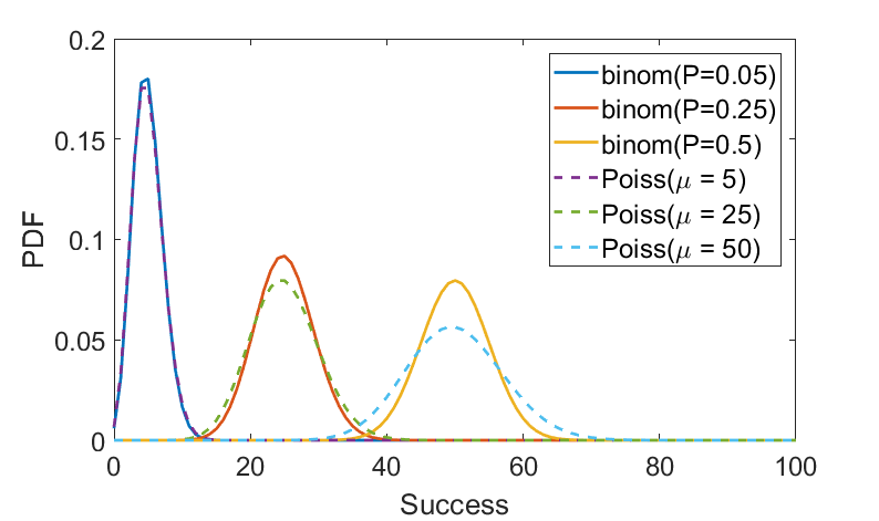
\end{aligned} \tag{4}$$ where in the last step, the approximation log (1−x) ∼  − x was utilized. As shown in Eq. 4, the limit of the Binomial distribution is the Poisson distribution when the number of trials is large over a fixed period T and the success probability is small. The mean number of events over the period T is often shown by μ = λT and hence the above result takes the following familiar form $$\mathrm{Poisson}(k;\mu) = \frac{\mu^k e^{-\mu}}{k!} \label{EqBi_5}\tag{5}$$ which is the Poisson distribution. Here, k is called increment of the process introduced before, also termed Poisson random variable.

Exponential Distribution

The waiting time between two consecutive Poisson events does not depend on the number of previous events or the events absolute times (axiom 2 in the Poisson Distribution section) and thus describes a memoryless process. Here, we show that such a memoryless process is an Exponential distribution.

To do so, we start by calculating the cumulative probability of an event happening up to a time t = T₁, given by

$$\begin{aligned} P(t\leq T_1)=1-(\mathrm{probability\, of\, no\, event\, for\,} t\leq T_1) \nonumber \\ = 1-\mathrm{Poisson}(k=0;\mu)=1-\frac{(\mu)^0}{0!}e^{-\mu} = 1-e^{-\lambda t}. \label{EqBi_6} \end{aligned} \tag{6}$$

This is the cumulative probability for the waiting time and therefore its derivative yields the probability distribution for the waiting time, which is the Exponential distribution $${\mathrm{Exponential}(t;\lambda)=\lambda e^{-\lambda t}.}\tag{7}$$ Since this result was derived given that the waiting time does not depend on locations of the events on the time axis in a Poisson process, the origin of time can be selected as the start of any waiting time and the above calculation holds for all the waiting times. Consequently, the time intervals between any two Poisson events follow an Exponential distribution.

Here, we demonstrate that any memoryless process defined on the interval [0, ∞) must be described by an Exponential distribution. To do so, we start by mathematical definition of a memoryless random variable t and then proceed to provide more explanaition and derive the distribution. A random variable t is memoryless if $${P(t>u+\nu|t>\nu)=P(t>u)}\tag{8}$$ for all positive values u and ν. This statement says that if an event has not taken place up to time ν, the probability that it does not happen for another time period u is described by the same probability distribution. This implies that if we move the origin of time to t = ν and assume that the waiting time starts there, the new waiting time also follows the same distribution. In other words, the system forgets that nothing has happened up to t = ν, i.e., memoryless. Using the Bayes formula, Eq. 8 can be written as $$P(t>u+\nu | t>\nu) = \frac{P(t>u+\nu,t>\nu)}{P(t>\nu)}=\frac{P(t>u+\nu)}{P(t>\nu)}. \tag{9}$$ Now, combining Eq. 8 and Eq. 9, one obtains $$P(t>u+v) =P(t>u)P(t>\nu).\tag{10}$$ The memoryless property is mathematically characterized by Eq. 10, which is satisfied by the exponential function $$P(t>u+v)=e^{-\lambda(u+\nu)} =e^{-\lambda u}e^{-\lambda \nu}=P(t>u)P(t>\nu).\tag{11}$$

by Mohamadreza Fazel