Gaussian Processes: An Intro to Nonparametric Regression

Introduction

In the world of machine learning, finding models that balance precision and flexibility is essential. Gaussian Processes (GPs) offer a captivating approach that thrives in the realm of nonparametric regression. With GPs, we venture beyond fixed assumptions, allowing uncertainty and adaptability to shine in our predictions. My goal here is to make this advanced topic approacahable and open the world of Statistical Learning for you. We will begin with some background and mathematical derivation, then move to a working example in python.

What are Gaussian Processes?

Gaussian Processes (GPs) are powerful Machine Learning tools that enable us to place probability distributions on all possible functions given the available data. Unlike traditional models with fixed parameters, GPs offer a statistical foundation for nonparametric regression. Instead of predicting individual points, GPs allow us to learn entire lines, surfaces, or even higher-dimensional functions. This remarkable capability lets us explore an infinite-dimensional space of functions, capturing complex relationships between inputs and outputs without being limited to rigid functional forms.

Applications of Gaussian Processes

Gaussian Processes find practical use in various domains:

• Nonparametric Regression: Embracing the nonparametric realm, GPs excel at modeling complex relationships without relying on predefined functional forms.

• Uncertainty Quantification: With GPs, we not only make predictions but also gain insights into the confidence and uncertainty surrounding those predictions. This is particularly valuable in scenarios with limited data or noisy observations.

• Bayesian Optimization: GPs guide us through the optimization of costly objective functions by effectively balancing exploration and exploitation.

• Time Series Analysis: GPs gracefully capture the intricate patterns hidden within time-dependent data, enabling accurate forecasting.

• Spatial Interpolation: In geostatistics, GPs serve as a reliable means to interpolate data over spatial domains, providing valuable spatial predictions.

• Active Learning: GPs play a key role in active learning, helping us choose the most informative points to query and thereby reducing the labeling effort.

Advantages and Limitations

Like any powerful tool, Gaussian Processes come with strengths and limitations:

Advantages:

Flexibility and Adaptability: GPs are masters of nonparametric regression, adapting to the intrinsic structure of the data. This flexibility enables them to achieve a more accurate fit than models with predefined functional forms.

Uncertainty Estimation: In a world filled with uncertainty, GPs offer a probabilistic perspective, providing not only point predictions but also measures of confidence around those predictions.

Data Efficiency: GPs perform well even with small datasets, efficiently utilizing the available information to make accurate predictions.

Interpretable Probabilistic Models: By modeling functions as random variables, GPs offer insights into the underlying relationships and allow us to interpret predictions more meaningfully.

Versatile Kernels: The choice of kernel allows customization to different data types and domain-specific knowledge, empowering users to capture diverse patterns in the data.

Limitations:

Computational Complexity: GPs can be computationally demanding, especially for large datasets. Inference and training may require significant computational resources.

Memory Intensity: Working with covariance matrices can be memory-intensive, impacting the scalability of GPs for large datasets.

Kernel Selection: The choice of the right kernel depends on the data and requires careful consideration and experimentation.

Curse of Dimensionality: GPs may face challenges in high-dimensional spaces, as the curse of dimensionality impacts their performance.

Global Optimization Challenges: GPs are non-convex models, making hyperparameter optimization a challenging task that requires careful exploration.

Mathematical Background

Review of Probability Distributions

Univariate Gaussian Distribution

The univariate Gaussian distribution, also known as the normal distribution, is a probability distribution defined for a single random variable. It is characterized by two parameters: the mean ($\mu$) and the variance ($\sigma^2$). The probability density function (PDF) of the univariate Gaussian is given by:

$$\mathcal{N}(x;\mu,\sigma^2) = \frac{1}{\sqrt{2\pi\sigma^2}} \exp\left(-\frac{(x-\mu)^2}{2\sigma^2}\right)$$

Where:

• $x$ is the random variable.
• $\mu$ is the mean, representing the expected value of $x$.
• $\sigma^2$ is the variance, defining the spread or variability of $x$.

The univariate Gaussian distribution is symmetric around its mean $\mu$, and its shape is determined by the variance $\sigma^2$. It is widely used in statistics and probability theory due to its many applications and mathematical properties.

Multivariate Gaussian Distribution

The multivariate Gaussian distribution generalizes the univariate Gaussian to multiple dimensions. Instead of dealing with a single random variable, we consider a random vector $\mathbf{x} = [x_1, x_2, \ldots, x_d]^T$ with $d$ dimensions. The multivariate Gaussian introduces two key components: the mean vector $\boldsymbol{\mu}$ and the covariance matrix $\boldsymbol{\Sigma}$.

In the multivariate Gaussian, the mean vector $\boldsymbol{\mu}$ represents the expected values of each component $x_i$. It defines the point in the multidimensional space around which the distribution is centered. The covariance matrix $\boldsymbol{\Sigma}$ captures the spread and correlations among the elements of $\mathbf{x}$. Each entry $\Sigma_{ij}$ of the covariance matrix represents the covariance between $x_i$ and $x_j$, indicating how the values of different components are related. If the elements of $\mathbf{x}$ are independent, the covariance matrix will be diagonal, with the variances of each component on the diagonal. However, if the elements are correlated, the covariance matrix will have non-zero off-diagonal elements.

The probability density function (PDF) of the multivariate Gaussian is defined as follows:

$$\mathcal{N}(\mathbf{x};\boldsymbol{\mu},\boldsymbol{\Sigma})=\frac{1}{(2\pi)^{d/2}\left|\boldsymbol{\Sigma}\right|^{1/2}}\exp\left(-\frac{1}{2}(\mathbf{x}-\boldsymbol{\mu})^\top\boldsymbol{\Sigma}^{-1}(\mathbf{x}-\boldsymbol{\mu})\right)$$

Where:

• $d$ is the dimension of the random vector $x$.
• $\mu$ is the mean vector, representing the expected value of $x$.
• $\Sigma$ is the covariance matrix, defining the spread and correlations among the elements of $x$.

To ensure the well-definedness of the multivariate Gaussian, the covariance matrix $\boldsymbol{\Sigma}$ must be positive definite. The multivariate Gaussian is a fundamental concept in Gaussian Processes, enabling us to model distributions over functions and capture complex relationships in data with multiple dimensions.

Gaussian Processes as Infinite-Dimensional Gaussians

Our exploration doesn’t end with finite-dimensional vectors; it leads us to the captivating realm of infinite-dimensional functions through Gaussian Processes. A Gaussian Process is essentially an infinite collection of random variables, where each function output $f(x)$ at any input $x$ follows a Gaussian distribution.

Imagine summoning an infinite number of functions, each characterized by a mean function $\mu(x)$ and a covariance function (kernel) $\mathbf{K}(x, x’)$. The mean function $\mu(x)$ defines the expected function output, while the covariance function $\mathbf{K}(x, x’)$ captures the relationships between the function outputs at inputs $x$ and $x’$.

The probability of function $f(x)$ in the world of Gaussian Processes is expressed as:

$$p(f(\mathbf{x});\boldsymbol{\mu}(\mathbf{x}), \mathbf{K}(\mathbf{x}, \mathbf{x’}))=\mathcal{N}\left(f(\mathbf{x});\boldsymbol{\mu}(\mathbf{x}), \mathbf{K}(\mathbf{x}, \mathbf{x’})\right)$$

Where:

• $f(x)$ is the function output at input x.
• $\mu(x)$ is the mean function, defining the expected function output.
• $\mathbf{K}(x, x’)$ is the covariance function (kernel), capturing the relationships between the function outputs at inputs x and x’.

What we have done here is come up with a way to assign a probability to any arbitrary function $f(x)$ based on the data $\mathbf{x}$. You can already see that our goal will be to find the function with the highest probability based on the data. Before we go about doing that, it is important to discuss the choice of the covariance function (kernel), as different kernels capture diverse patterns and structures in the data. Gaussian Processes provide a powerful framework for non-parametric regression, enabling us to model complex functions and make predictions based on limited observations. As we delve deeper into the fascinating world of covariance functions, we gain a deeper understanding of the flexibility and versatility of Gaussian Processes in handling various real-world problems.

Positive Definite Kernels

To ensure that the covariance matrix $\mathbf{K}$ remains positive definite, and thus ensures a valid Gaussian distribution, the kernel must satisfy the positive definiteness property. A kernel function $k(\mathbf{x}, \mathbf{x’})$ is positive definite if, for any finite set of points $\{\mathbf{x}_1, \mathbf{x}_2, …, \mathbf{x}_m\}$, the associated matrix $\mathbf{K}$ of size $m \times m$ is positive definite. In mathematical terms, this property is expressed as:

$$\sum_{i=1}^{m} \sum_{j=1}^{m} c_i c_j k(\mathbf{x}_i, \mathbf{x}_j) \geq 0$$

for any choice of real coefficients $c_1, c_2, …, c_m$.

Commonly Used Covariance Functions

In the vast magical repertoire of covariance functions, some widely used kernels include:

1. Radial Basis Function (RBF) Kernel (Squared Exponential Kernel)

The RBF kernel, also known as the Squared Exponential kernel, is defined as:

$$k_{RBF}(\mathbf{x}, \mathbf{x’}) = \sigma^2 \exp\left(- \frac{||\mathbf{x} – \mathbf{x’}||^2}{2l^2}\right)$$

Where:

• $||\mathbf{x} – \mathbf{x’}||^2$ represents the squared Euclidean distance between the input points $\mathbf{x}$ and $\mathbf{x’}$.
• $\sigma^2$ is the variance parameter that controls the overall amplitude or scale of the kernel.
• $l$ is the length scale hyperparameter that controls the smoothness of the functions. Large $l$ values result in smoother functions, while smaller values lead to more wiggly functions.

2. Matérn Kernel

The Matérn kernel is a family of kernels, characterized by an additional parameter $\nu$ that controls the level of smoothness:

$$k_{Matern}(\mathbf{x}, \mathbf{x’}) = \frac{2^{1-\nu}}{\Gamma(\nu)} \left(\frac{||\mathbf{x} – \mathbf{x’}||}{l}\right)^\nu B_\nu\left(\frac{||\mathbf{x} – \mathbf{x’}||}{l}\right)$$

Where $Gamma(\nu)$ is the gamma function, and $B_\nu(\cdot)$ is a modified Bessel function of the second kind.

3. Linear Kernel

The linear kernel captures linear relationships between inputs and is defined as:

$$k_{Linear}(\mathbf{x}, \mathbf{x’}) = \mathbf{x}^\top \mathbf{x’}$$

4. Periodic Kernel

The Periodic kernel introduces periodicity to the model and is defined as:

$$k_{Periodic}(\mathbf{x}, \mathbf{x’}) = \sigma^2 \exp\left(-2 \sin^2\left(\frac{\pi ||\mathbf{x} – \mathbf{x’}||}{p}\right) / l^2\right)$$

Where:

• $||\mathbf{x} – \mathbf{x’}||$ represents the distance between the input points $\mathbf{x}$ and $\mathbf{x’}$.
• $\sigma^2$ is the variance parameter that controls the overall amplitude or scale of the periodic variations.
• $l$ is the length scale hyperparameter that controls the smoothness of the periodic behavior.
• $p$ is the hyperparameter that determines the period of the kernel.

The Periodic kernel is particularly useful for modeling data with repeating patterns or cyclic behavior.

Choosing the Right Covariance Function

Selecting the right covariance function is an artful task, as it profoundly impacts the model’s performance. The choice depends on the data’s properties, the expected smoothness, the presence of periodic behavior, and the patterns to capture. Experimentation and careful consideration of domain knowledge guide the journey to finding the most suitable and magical covariance function for a particular application.

In the world of Gaussian Processes, covariance functions grant us the power to wield the magic of nonparametric regression, where uncertainty is embraced, adaptability thrives, and the variance parameter, length scale, and periodicity control the amplitude, smoothness, and cyclical behavior of the enchanting functions. With the right choice of kernels, we traverse a realm of infinite-dimensional functions, capturing the mysteries hidden within our data.

Derivation of Conditional Distribution (Non-Zero Mean GP)¹

Given the joint distribution of the training outputs $\mathbf{y}$ and the test outputs $\mathbf{y^*}$:

$$\begin{bmatrix} \mathbf{y} \\ \mathbf{y^*} \end{bmatrix} \sim \mathcal{N}\left(\begin{bmatrix} \mathbf{m}(\mathbf{X}) \\ \mathbf{m^*}(\mathbf{X^*}) \end{bmatrix}, \begin{bmatrix} \mathbf{K} & \mathbf{K}(\mathbf{X}, \mathbf{X^*}) \\ \mathbf{K}(\mathbf{X^*}, \mathbf{X}) & \mathbf{K}(\mathbf{X^*}, \mathbf{X^*}) \end{bmatrix}\right)$$

Where:

• $\mathbf{m}(\mathbf{X})$ is the mean vector of size $n \times 1$ at the training data points.
• $\mathbf{m^*}(\mathbf{X^*})$ is the mean vector of size $m \times 1$ at the test data points.

We want to find the conditional distribution $\mathbf{y^*} | \mathbf{X}, \mathbf{y}, \mathbf{X^*}$. The conditional distribution of a multivariate Gaussian can be expressed as:

$$P(\mathbf{y^*} | \mathbf{X}, \mathbf{y}, \mathbf{X^*}) = \mathcal{N}(\mathbf{\mu^*}, \mathbf{K^*})$$

where $\mathbf{\mu^*}$ and $\mathbf{K^*}$ are the mean vector and covariance matrix of the conditional distribution, respectively.

Step 1: Finding the Conditional Mean $\mathbf{\mu^*}$

The conditional mean $\mathbf{\mu^*}$ can be computed using the properties of conditional expectation:

$$\mathbf{\mu^*} = \mathbb{E}[\mathbf{y^*} | \mathbf{X}, \mathbf{y}] = \mathbb{E}[\mathbf{y^*} | \mathbf{X}, \mathbf{y}, \mathbf{X^*}]$$

To find $\mathbf{\mu^*}$, we need to compute the conditional expectation $\mathbb{E}[\mathbf{y^*} | \mathbf{X}, \mathbf{y}, \mathbf{X^*}]$ given that $\mathbf{y}$ is observed.

The conditional distribution is computed using the formula for conditional Gaussian distributions:

$$\mathbf{\mu^*} = \mathbf{m^*}(\mathbf{X^*}) + \mathbf{K}(\mathbf{X^*}, \mathbf{X}) \mathbf{K}^{-1}(\mathbf{X}, \mathbf{X}) (\mathbf{y} – \mathbf{m}(\mathbf{X}))$$

Step 2: Finding the Conditional Covariance $\mathbf{K^*}$

The conditional covariance $\mathbf{K^*}$ can be computed using the formula for conditional variance:

$$\mathbf{K^*} = \text{Var}[\mathbf{y^*} | \mathbf{X}, \mathbf{y}] = \mathbf{K}(\mathbf{X^*}, \mathbf{X^*}) – \mathbf{K}(\mathbf{X^*}, \mathbf{X}) \mathbf{K}^{-1}(\mathbf{X}, \mathbf{X}) \mathbf{K}(\mathbf{X}, \mathbf{X^*})$$

Let’s break down the equation step by step:

• $\mathbf{K^*}$ is the covariance matrix of size $m \times m$ representing the uncertainty in the predicted outputs at the test points.
• $\mathbf{K}(\mathbf{X^*}, \mathbf{X^*})$ is the covariance matrix of size $m \times m$ for the test points.
• $\mathbf{K}(\mathbf{X^*}, \mathbf{X})$ is the covariance matrix of size $m \times n$ between the test points and the training points.
• $\mathbf{K}(\mathbf{X}, \mathbf{X^*})$ is the covariance matrix of size $n \times m$ between the training and test points, where $n$ is the number of training points.

By computing $\mathbf{K^*}$, we obtain the covariance matrix that quantifies the uncertainty in the predictions at the test points, accounting for the information from the training data $\{\mathbf{X}, \mathbf{y}\}$ and the non-zero mean functions $\mathbf{m}(\mathbf{X})$ and $\mathbf{m^*}(\mathbf{X^*})$.

Thus, we have derived the conditional distribution of the test outputs $\mathbf{y^*}$ given the training data $\mathbf{X}$ and $\mathbf{y}$, which is represented by the multivariate Gaussian $\mathcal{N}(\mathbf{\mu^*}, \mathbf{K^*})$. These equations provide us with the predictive mean and covariance at the test points, allowing us to make predictions and quantify the uncertainty of the Gaussian Process Regression model with non-zero mean functions.

Gaussian Process Regression with Synthetic Data

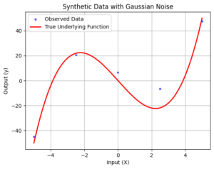
In this tutorial, we’ll explore Gaussian Process Regression using synthetic data generated from a cubic polynomial function with added Gaussian noise. We’ll visualize the data, define the squared exponential kernel and covariance matrix, and perform Gaussian Process Regression to predict the underlying function and its uncertainty.

1. Generate Synthetic Data

We start by generating synthetic data. We define the true underlying cubic polynomial function truePolynomial(x) and create observed data points with random Gaussian noise. The data is visualized to observe the true underlying function along with the noisy observed data points.

#Necessary Imports
import numpy as np
import matplotlib.pyplot as plt

# Set random seed for reproducibility
np.random.seed(42)

# Define the true underlying polynomial function
def truePolynomial(x):
    y = x**3 - 15 * x
    return y

#Define Ground Truth and Generate synthetic data
x = np.linspace(-5, 5, 10000)
y = truePolynomial(x)
xData = np.linspace(-5, 5, 5)
yData = truePolynomial(xData) + 10 * np.random.randn(len(xData))

# Visualize the data
plt.scatter(xData, yData, label='Observed Data', color='b', alpha=0.6, s=10)
plt.plot(x, y, label='True Underlying Function', color='r', linewidth=2)
plt.xlabel('Input (X)')
plt.ylabel('Output (y)')
plt.legend()
plt.title('Synthetic Data with Gaussian Noise')
plt.grid(True)
plt.show()

2. Define the Squared Exponential Kernel and Covariance Matrix

Next, we define the squared exponential kernel function and the covariance matrix generator function. The squared exponential kernel measures the similarity between data points, and the covariance matrix stores the similarities between training and test points. These functions will be used in the Gaussian Process Regression.

# Define the squared exponential kernel function
def squaredExpKernel(x1, x2, sigma=1.0, lengthScale=1.0):
    val = (sigma**2) * np.exp(-0.5 * ((x2 - x1) / lengthScale)**2)
    return val

# Define the covariance matrix generator function
def covMatGenerator(v1, v2, sigma=1, lengthScale=1):
    K = np.zeros((len(v1), len(v2)))
    for i in range(len(v1)):
        for j in range(len(v2)):
            K[i, j] = squaredExpKernel(v1[i], v2[j], sigma, lengthScale)
    return K

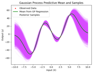
3. Perform Gaussian Process Regression

Now, we perform Gaussian Process Regression on the synthetic data. We generate test points and calculate the covariance matrices for training and test points. To ensure numerical stability, we regularize the covariance matrix for training points. Using the training data and the covariance matrices, we predict the output at test points and calculate the uncertainty or confidence intervals. Finally, we generate samples from the posterior using the multivariate normal generator.

# Generate test points
xTest = np.linspace(-10, 10, 100)

# Generate the covariance matrices for training and test points
KTrainTrain = covMatGenerator(xData, xData, 10, 2)
KTestTrain = covMatGenerator(xTest, xData, 10, 2)
KTestTest = covMatGenerator(xTest, xTest, 10, 2)

# Regularize the covariance matrix for numerical stability
KTTInv = np.linalg.inv(KTrainTrain + 1e-3 * np.eye(len(KTrainTrain)))

# Predict the output at test points and calculate the uncertainty
yTest = KTestTrain @ (KTTInv @ yData)
kTest = KTestTest - KTestTrain @ (KTTInv @ KTestTrain.T)

# Generate samples from the posterior using multivariate normal generator
samples = np.random.multivariate_normal(yTest, kTest, 10000).T

#Visualize the Samples
plt.plot(xTest, samples, color='#d84bff', alpha=0.1)  # Plot empty data just for the label
plt.scatter(xData, yData, c='r', s=10, label='Observed Data')
plt.plot(xTest, yTest, color='g', linewidth=2, label='Mean from GP Regression')
plt.plot([], [], color='#d84bff', alpha=0.1, label='Posterior Samples')
plt.legend()
plt.title('Gaussian Process Predictive Mean and Samples')
plt.xlabel('Input (X)')
plt.ylabel('Output (y)')
plt.show()

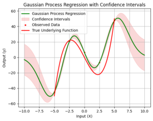
4. Visualize Gaussian Process Regression with Confidence Intervals

Finally, we visualize the results of Gaussian Process Regression along with the confidence intervals. The green curve represents the Gaussian Process Regression, and the shaded region around it shows the confidence intervals. The width of the shaded area indicates the uncertainty associated with our model’s predictions. We can observe how well the Gaussian Process captures the true underlying function and how the uncertainty varies at different points.

# Calculate the standard deviation at each test point to obtain confidence intervals
std_dev = np.std(samples, axis=1)

# Plot the Gaussian Process Regression with Confidence Intervals
plt.plot(xTest, yTest, label='Gaussian Process Regression', color='g', linewidth=2)
plt.fill_between(xTest, yTest - 2 * std_dev, yTest + 2 * std_dev, color='lightcoral', alpha=0.3, label='Confidence Intervals')
plt.scatter(xData, yData, c='r', s=10, label='Observed Data')
plt.plot(x, y, label='True Underlying Function', color='r', linewidth=2)
plt.xlabel('Input (X)')
plt.ylabel('Output (y)')
plt.legend()
plt.title('Gaussian Process Regression with Confidence Intervals')
plt.grid(True)
plt.show()

In conclusion, Gaussian Processes offer a powerful approach for nonparametric regression with advantages like flexibility, uncertainty quantification, and interpretable probabilistic models. However, as datasets grow larger, the computational burden of GPs becomes a significant challenge. The matrix inversion required in GP computations and the limitations of built-in samplers can hinder scalability for large datasets. In our upcoming blog, we will explore effective strategies to address these issues and make Gaussian Processes computationally feasible for handling massive data. We will delve into kernel-based approximation techniques, which provide an alternative to traditional matrix inversion approaches. Additionally, we will discuss sparse approximations, which allow us to work with reduced representations of data and significantly improve computational efficiency while preserving the core properties of GPs. By understanding these techniques and finding the right balance between approximation and model accuracy, we can harness the full potential of Gaussian Processes even with large datasets. Stay tuned to learn how to mitigate the computational expense of GPs and unleash their power for big data applications!