The Matrix exponential

Consider a vector-valued function $\vec{v}(t)$ whose total derivative with respect to its argument is given explicitly by a linear operator $A$ (which we’ll represent as a matrix):
$$\frac{d\vec{v}(t)}{dt} = \vec{v}(t) A .$$

Suppose at some $t$ we know the function’s value $\vec{v}(0)$. (N.B. We’ve chosen $t=0$ here without losing generality; for any finite non-zero $t$ we can recover $t=0$ through a trivial change of variables $t \rightarrow t-t_0$).

We can Taylor expand $\vec{v}$ at some later time $t_f$

$$\vec{v}(t_f) = \sum_{n=0}^{\infty} \frac{1}{n!}(t)^n\left(\frac{d}{dt}\right)^n \vec{v}(t_f)$$

and simply substitute the action of the derivative for its matrix equivalent $\frac{d}{da}(\cdot) = \cdot \times A$:

$$\vec{v}(t_f) = \sum_{n=0}^{\infty} \frac{1}{n!}\vec{v}(t_f)(tA)^n = \vec{v}(0) \left(\sum_{n=0}^{\infty} \frac{1}{n!}(tA)^n\right) .$$

To anyone familiar with the Taylor series for the exponential of a scalar, this series ought to look familiar. In fact, if $\vec{v}$ is one-dimensional, $A$ is a $1\times1$ matrix, and $e^{tA}$‘s one element is given by the scalar exponential of $a$ times $A$‘s only element. Therefore, since $\vec{v}(0)$ is independent of $n$, we can represent the sum as a single operator $$e^{tA} = \sum_{n=0}^{\infty} \frac{1}{n!}(tA)^n ,$$ which is aptly named the exponential of the matrix $tA$

Krylov Subspaces

Now that we know the matrix exponential’s role and its definition, we turn briefly to the general topic of Krylov subspaces, before explaining how they help us to compute matrix exponentials.

Why Krylov Subspaces for Matrix Exponentiation

A number of open problems in science ultimately amount to exponentiating large matrices, sometimes repeatedly. Although a variety of methods to accelerate matrix exponentials exist, the Krylov exponential is attractive for a few reasons:

1. Elegance: The Krylov subspace method reduces a linear problem’s dimensionality meaningfully, utilizing the problem itself to extract the proper reduced-order features.
2. Speed: the Krylov subspace exponential has been proven efficient for exponentiating matrices both in terms of absolute time and time cost scaling
3. Storage: Since it only uses matrix-vector products, if the matrix being exponentiated can be efficiently stored as a sparse matrix, it requires vastly less storage allocations than naive approaches.

Here, I’ll go through a detailed explanation of the algorithm (complete with Julia code) and elaborate on each of the points 1-3 above, along with some of its potential downsides.

What are they?

Simply defined and powerful in their applications, an order-$\kappa$ Krylov subspace of $A$ and $\vec{v}$ is given by

$$\mathcal{K}_{\kappa}(A,\vec{v}) = span\{\vec{v},A\vec{v},A^2\vec{v},\dots,A^{\kappa}\vec{v}\}$$

that is, the space spanned by vectors obtained by applying successive powers of $A$ to the vector $\vec{v}$. Although these matrix-vector products give an acceptable basis for $\mathcal{K}_{\kappa}(A,\vec{v})$, manipulating the projection of $A$ into $\mathcal{K}_{\kappa}(A,\vec{v})$ will be much easier if we obtain it in an orthonormal basis.

Arnoldi Algorithm

The Arnoldi Algorithm (or Arnoldi Iteration) is a simple method for obtaining an orthonormal basis, $\{\vec{q}_1,\vec{q}_2,…\}$, along with a projection of a matrix (in our case, $A$, the one we want to exponentiate) into that basis. We will use the basis vectors as the columns of a matrix $\mathbf{Q} = [\vec{q}_1,\vec{q}_2,…]$, and refer to the projection of $A$ as $H$.

# Inputs: the vector (v), the matrix (A), and the dimensionality of the subspace (k)
# Outputs: The projection H and the basis vectors, as the columns of Q
function get_arnoldi(v,A,κ)
    H = zeros(Float32,κ,κ)          # Initialize the outputs
    Q = zeros(Float32,length(v),κ)  
    Q[:,1] = v/norm(v)              # Set the first basis vector
    for k = 2:κ
        Q[:,k] = view(Q,:,k-1)'*A   # Initialize each q_k basis vector
            for l = 1:k-1           # For each previous vector in Q
                H[l,k-1] = dot(Q[:,l],Q[:,k]) # Compute the appropriate matrix projection element
                Q[:,k]  -= H[l,k-1]*Q[:,l]    # Subtract all components of q_k that aren't orthogonal
            end
        H[k,k-1] = norm(Q[:,k])
        Q[:,k]  /= H[k,k-1] # Normalize q_k 
    end
    return H, Q
end

Now, assuming it $A$ is captured well by its action within the subspace,
$$A = Q^THQ.$$

In reality, this equation is only approximate, with approximation error that depends on the subspace size $\kappa$, as we’ll see later. Since Q is an orthonormal matrix, we can now write the exponential of $A$ (using $Q^{T}Q = \mathbb{I}$) as

$$e^{A} \approx e^{Q^{T}HQ} = Q^{T} e^{H} Q.$$
And that should be all we need, right? To check and see, let’s look at some examples…

Linear ODE Example: The CME

For Markovian stochastic systems evolving in continuous time through a discrete state space, the time-evolving probability of the system’s states is given by a set of linear ODEs referred to as the Chemical Master Equation (CME for short):
$$\frac{d \vec{\rho}(t) }{dt} = \vec{\rho}(t) G.$$

Here, each element of the vector $\vec{\rho}$ is the probability of the system occupying each state. If our system can occupy $I$ distinct states, we can enumerate them as $\sigma_i$, so that $\vec{\rho}(t)$ has elements
$$\vec{\rho}(t)_i = p(\sigma_i|t)$$

which give the probability that the system occupies each state at a given time. The matrix $G$, known as the “generator matrix”, is made up primarily of the transition rates between states

$$G_{jk} = \lambda_{j \rightarrow k} \; \text{for} \; j \neq k.$$

Then the diagonal elements are specified to guarantee probability conservation (that is, so that its rows sum to 1)

$$G_{jj} = -\sum_{k\neq j}\lambda_{j \rightarrow k}.$$

Death system

Perhaps the simplest example of these dynamics is a reaction network which consists of some number (let’s call it $r$) of copies of a single species, which has a population between $0$ and $R$. It may seem concocted, but these dynamics are particularly important for describing the population of a species under radioactive decay.

In each infinitesimal $dt$, each individual has a probability $\gamma dt$ of dying. In the language of chemical reactions:
$$r \overset{\gamma}{\rightarrow} \empty.$$

In this process, the generator matrix then has off-diagonal elements:
$$G_{ij} = i \gamma \;\; \text{if} \;\; i-j=1,$$
$$G_{ij} = 0 \;\; \text{otherwise},$$
with $G_{jj}$ given as above.

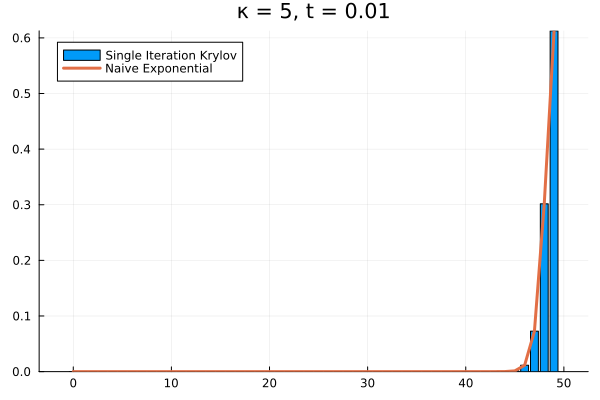
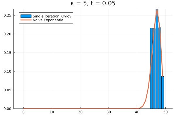
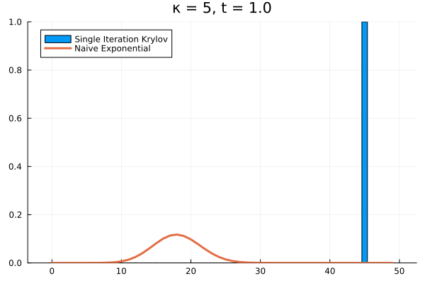
For example, if we arbitrarily set the initial population to $50$ and $\gamma = 1$, the short time behavior is captured well by the Krylov exponential

Saving the Krylov Exponential

The Naive Approach

Clearly, our method needs saving. What if we try increasing $\kappa$ to $10$?

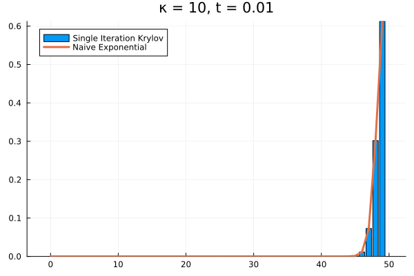
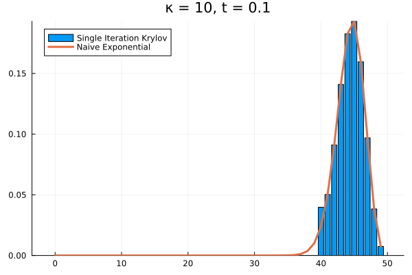
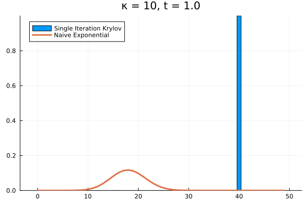
As it turns out, we’re seeing the effect of $H$ being the projection of $A$ into $\mathcal{K}_k(A,\vec{v}(0))$. The exponential of our projection $H$ represents the dynamics over the time interval as the superposition of $\vec{v}(0)$ times powers only up to $A^\kappa$. If we look at the structure of $A$, it’s clear that applying it to any vector with all the probability mass concentrated in once state can only result in increasing the probability in the adjacent state. Then each successive application of $A$ shifts density one state further, eventually limited by $\kappa$, the number of applications of $A$. The result is that for our example above, the solution has to have all its density in the states $\sigma_{R-5}\dots\sigma_R$.

The problem persists even if we increase $\kappa$ further.

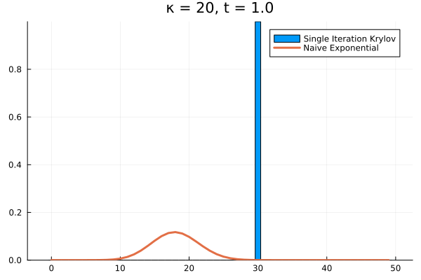
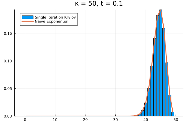
Evidently, we’re still limited by our (now increased) $\kappa$. This means that in order to track the probability density over all the states of our system, we would need to increase $\kappa$ to $R$, and the resulting Krylov subspace doesn’t reduce the size of our eventual matrix exponential at all!

Only Use Short Time Intervals

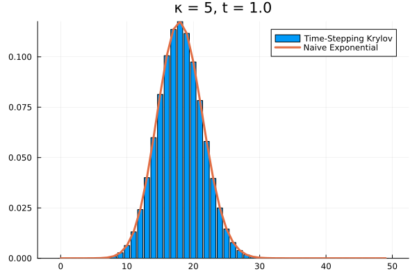
Ok, so reducing the complexity of computing our matrix exponential has the cost of reducing the complexity of the changes we can make to our initial vector. As it turns out, we can still save our method by relying only on simple changes to our initial vector if we split our time evolution into small steps. As with other differential equation solving methods (Euler Method, Runge-Kutta, etc.), the Krylov exponential now becomes an incremental time-stepping approach:

$$\vec{v}(t+dt) = \vec{v}(t)e^{Gdt} .$$

# Inputs: the initial vector (v), the matrix (A), the dimensionality of the subspace (k), the time-span for integration (t_span), and the time-step (dt)
# Outputs: The final, transformed vector (v)
function krylov_exp(v,A,κ,t_span,dt)
    # If the time grid doesn't end at the final time, append it to the time grid
    t_grid = t_span[1]:dt:t_span[2]
    # Purge and non-unique elements from the time grid
    t_grid = unique(vcat(t_grid,t_span[2]))
    # Iterate over time grid
    for i  = Base.OneTo(length(t_grid)-1)
        # Compute time interval
        Δt = t_grid[i+1]-t_grid[i]
        # Arnoldi iteration to obtain H,Q
        H,Q = get_arnoldi(v,A,κ)
        # Recover the exponential
        v = norm(v) * (Q * exp(H*Δt))[:,1]
        # And guarantee it's normalized
        v/=sum(v)
    end
    return v
end

Choosing a time step of $dt = 0.01$, we can recover the full time evolution of our death system to its equilibrium.

Conclusions

Although they seem at first to promise a complete side-stepping of the full dimensional matrix exponential, Krylov subspaces are most suitable for use within a time-stepping approach, like Runge-Kutta or the Euler method. They have the distinct advantage of reducing the problem’s dimensionality, in a well-reasoned manner, and proceeding accordingly.

As we’ll explore further in my next post, the Krylov subspace approach increases the speed and reduces the storage requirements of the exponential of sparse matrices sparse matrices in particular, by reducing the problem’s dimensionality. It does this with the elegant insight that right space for a propagated vector to live in is spanned by that vector times successive powers of the matrix (i.e. the Krylov subspace). For a more detailed analysis of the Krylov Exponential, check out a recently released article, in which we utilized some benchmarking principles (described by my co-author in a recent blog post) to compare the Krylov matrix exponential to three additional methods for avoiding direct matrix exponentiation.

Next Up: More Complicated Dynamics and QM time evolution

With the death system, we have barely scratched the surface of the matrix exponential’s potential. Next time, we’ll look at more general reaction dynamics, larger state-spaces, and more reaction pathways.

Furthermore, we’ve framed the present discussion in terms of real-valued vector functions and real matrices, but it applies equally to complex vector spaces. Therefore next time, we’ll discuss the role of the matrix exponential in quantum mechanics, and review some examples which involve computing complex amplitudes with matrix exponentials of Hermitian operators.