Gaussian Processes: Harnessing the Bayesian Paradigm

Gaussian Processes (GPs) stand as an embodiment of Bayesian principles in the realm of machine learning and probabilistic modeling. Today we begin a mathematical voyage to show the integration of Gaussian Process Regression within the Bayesian framework. This exploration will unravel the inherent connections between Gaussian Processes and Bayes’ theorem, delve into the complexities of non-conjugate likelihoods, and culminate in a tangible example with python. We will focus sepcifically on the integration od GPs within a Bayesian paradigm, so if you are unfamiliar with Gaussian Processes check out my introductory post here where I dive into their mathematical structure and role in regression.

The Gaussian Process in Context of Bayes’ Theorem: An Analytical Duet

Bayes’ Theorem: Formal Prelude

I don’t want to jump into the debate of a Frequentist vs. Bayesian paradigm, as they both have their own benefits and pitfalls, but I do want to properly motivate Bayesian Inference. Whenever you have a statistical model describing a set of observation, data, you are able to assign a probabilities to the observations given a set of model parameters. Usually it is quite simple to identify a set model parameters that maximize the probability of the data, this is known as a Maximum Liklihood Estimate, MLE. While this framework is very good for data summarization, it only provides point estimates, which tends to overfit at lower quantities of data, thus motivating a framework that can estimate probable parameters while also quantifying uncertaintity and reliability of fit. At the heart of Bayesian inference lies Bayes’ theorem, a probabilistic embodiment of the relation between the data and the model parameters. Specifically, it provides a framework to assign probabilities to all possible parameters given a set of data, allowing for better uncertainty quantification. Symbolically, Bayes’ theorem takes the form:

$$P(\text{Parameters}\,|\,\text{Data}) = \frac{P(\text{Data}\,|\,\text{Parameters}) \cdot P(\text{Parameters})}{P(\text{Data})}$$

In this equation:

• $P(\text{Parameters}\,|\,\text{Data})$ signifies the posterior probability of the parameters given the data.
• $P(\text{Data}\,|\,\text{Parameters})$ represents the likelihood of the data given the model parameters.
• $P(\text{Parameters})$ is the prior probability assigned to the model parameters.
• $P(\text{Data})$ denotes the probability of the observed data.

Fusion of Concepts: Gaussian Process and Bayes

Now one might be asking where does a GP fit into all of this. Alot of times the model parameters we are trying to learn are not a single values, but rather entire functions. Assigning probabilities to entire functions or data distributions, while encompassing initial beliefs, is exactly what Gaussian Processes do. Thus it is natural to use them as a prior for any multivariate model parameters. Additionally, when used as a prior on a model with a Gaussian likelihood, the posterior distribution itself takes the form of a GP. Fundamental to Bayesian inference and Gaussian Processes is marginalization. Just as Bayesian inference requires integration over nuisance parameters, Gaussian Processes involve integration over unobserved function values. This crucial step employs multivariate Gaussian distributions, streamlining integration and providing posterior predictions. The Gaussian Process framework thus seamlessly incorporates the foundational components of Bayes’ theorem, transforming them into a framework accommodating continuous functions and probabilistic uncertainty.

The Gaussian Process Prior: Unveiling Insights

In Bayesian inference, the Gaussian Process (GP) prior serves as a cornerstone, imparting distinctive attributes to Gaussian Processes and allowing them to encapsulate function uncertainty. This section embarks on a mathematical exploration of the Gaussian Process prior, delving into its intricacies and implications.

Revealing the Gaussian Process Prior with an Arbitrary Mean

At its core, the Gaussian Process prior offers a probabilistic perspective on function understanding. Rather than specifying a single deterministic function, a Gaussian Process defines an infinite ensemble of functions, linked through a multivariate Gaussian distribution. This distribution operates in function space, encapsulating beliefs about function behavior across diverse input points.

Mathematically, a Gaussian Process can be formulated with an arbitrary mean function$m(x)$:

$$f(x) \sim \mathcal{GP}(m(x), k(x, x’))$$

Where:

• $f(x)$ is the latent function of interest.
• $m(x)$ signifies the arbitrary mean function, incorporating prior beliefs or domain expertise.
• $k(x, x’)$ is the kernel function, capturing covariance between function values at distinct input points.

The Gaussian Process stipulates that the vector $\mathbf{f} = [f(x_1), f(x_2), \ldots, f(x_n)]^T$ follows a multivariate Gaussian distribution:

$$\mathbf{f} \sim \mathcal{N}(\mathbf{m}, K)$$

Where:

• $\mathbf{m} = [m(x_1), m(x_2), \ldots, m(x_n)]^T$ denotes the vector of mean function values.
• $K$ represents the kernel matrix, capturing covariance between function values at different input points.

Epistemic Foundations: Correlation and Uncertainty

The kernel matrix$K$assumes a pivotal role within the Gaussian Process, encoding beliefs about relationships between function values. Through its structure, the kernel governs interactions between diverse input points, influencing GP smoothness, periodicity, and other critical characteristics. This kernel establishes a probabilistic framework translating intuitions into the realm of functions.

This epistemic perspective profoundly shapes machine learning approaches. It empowers us to account for both data uncertainty and the inherent uncertainty of underlying functions. By selecting kernel functions and hyperparameters judiciously, we can tailor Gaussian Processes to domain knowledge and model assumptions.

Building the Foundation: Prior-Predictive Distribution

The essence of the Gaussian Process prior is fully revealed through the prior-predictive distribution. This distribution combines the GP prior with insights from observed data. By augmenting the prior with data, we interpolate between prior beliefs and evidence provided by observations. This amalgamation can be expressed as:

$$P(\mathbf{f} \,|\, X) = \int P(\mathbf{f} \,|\, X, \boldsymbol{\theta}) \cdot P(\boldsymbol{\theta} \,|\, X) \, d\boldsymbol{\theta}$$

Where:

• $X$ signifies input data.
• $\mathbf{f}$ represents the vector of function values.
• $\boldsymbol{\theta}$ corresponds to hyperparameters governing the kernel and likelihood.

Through the prior-predictive distribution, the Gaussian Process prior accommodates empirical evidence, refining behavior while acknowledging the interplay of uncertainty and information.

We have unraveled the crucial role of the Gaussian Process prior with an arbitrary mean in grasping Gaussian Processes within the Bayesian framework. Its influence on shaping the understanding of functions, managing uncertainty, and embracing domain expertise underscores the profound harmony between Gaussian Processes and Bayesian principles. This foundation sets the stage for our upcoming exploration of the intricate interaction between Gaussian Processes and non-conjugate likelihoods, culminating in a comprehensive grasp of probabilistic modeling and inference.

Integrating with Gaussian Likelihood: Synthesis of Data and Function

The seamless integration of Gaussian Processes (GPs) into the Bayesian framework presents a robust approach to harmonizing prior beliefs with observed data. This synthesis yields a modeling technique characterized by flexibility and principled foundations, allowing Gaussian Process priors and Gaussian likelihoods to seamlessly combine.

Intersecting Priors and Likelihoods: The Gaussian Process Posterior

Central to Bayesian analysis is the pursuit of revealing latent functions $f(x)$ through a balance between prior assumptions and empirical evidence. This quest culminates in the derivation of the posterior distribution, denoted as $P(f(x) \,|\, D)$ , where $D$ represents observed data. The framework for constructing this pivotal distribution rests upon Bayes’ theorem:

$$P(f(x) \,|\, D) = \frac{P(D \,|\, f(x)) \cdot P(f(x))}{P(D)}$$

Within Gaussian Process regression, the conjugacy of a Gaussian likelihood and Gaussian Process prior yields an analytically manageable and cohesive posterior distribution. When the Gaussian likelihood term $P(D \,|\, f(x))$ takes the form of a Gaussian distribution, it embodies a mean $f(x)$ and variance $\sigma_{\text{data}}^2$ , indicating noise variability associated with observations. This choice of Gaussian likelihood is especially suited for scenarios with diverse and uncorrelated sources of uncertainty, resembling general white noise characteristics. This approximation enables effective modeling of various noise types, making it a widely adopted technique in contexts like sensor measurements, financial market fluctuations, and communication channel noise.

Specifically, the Gaussian likelihood term $P(D \,|\, f(x))$ assumes the shape of:

$$P(D \,|\, f(x)) = \mathcal{N}(f(x), \sigma_{\text{data}}^2)$$

The resulting posterior distribution, a consequence of conjugacy, adopts the form:

$$P(f(x) \,|\, D) = \mathcal{N}(\mu_{\text{post}}, \sigma_{\text{post}}^2)$$

This derivation is done in the previous blog post. This framework unveils several key aspects:

• $\mu_{\text{post}}$ , representing the posterior mean of latent function$f(x)$, amalgamates the prior mean and data-driven predictions.
• $\sigma_{\text{post}}^2$ , denoting posterior variance, encapsulates the intricate interaction between prior assumptions and empirical observations, quantifying ensuing uncertainty.

Crucially, when likelihood aligns harmoniously with the Gaussian distribution, Gaussian Process regression transitions seamlessly into the realm of Gaussian regression. The case of a normal likelihood mirrors standard Gaussian Process regression, as demonstrated above. This case is further elaborated in my previous blog post.

Non-Conjugate Likelihoods: Navigating Complexity

Beyond the Gaussian Veil: Diverse Likelihood Domains

The application of Gaussian Process (GP) models extends beyond Gaussian likelihoods, encompassing a wide array of probabilistic scenarios. While Gaussian likelihoods provide analytical convenience, the stochastic modeling encompasses a multitude of data generation processes. These involve data emissions governed by various distributions both continuous and discrete. It’s important to note that the likelihood function can take any shape accurately characterizing the relationship between observed data and the latent function. Thus it is easy to find yourself in a situation where you want to use a Gaussian Process prior to allow for inference of entire functions, but your liklihood is not Gaussian. To ease any fears, I should say not much changes, you still have a posterior distribution given by Bayes’ Theorem that assign probabilities to all possible parameters. The lack of conjugacy between prior and liklihood necessitates numerical simulation.

Strategies for Non-Conjugate Inference

Effectively addressing non-conjugate likelihoods involves various deterministic and stochastic optimization techniques. You can use them interchangeably depending on wether you want to simply maximize your posterior, find the most probable parameters, or generate samples for rigorous uncertainty quantification.

Deterministic Techniques:

• Gradient Descent: A foundational method iteratively refining model parameters by descending along the gradient of the chosen objective function. It seeks parameter values minimizing the discrepancy between model predictions and observed data.
  • Pros: Simple implementation, computational efficiency for moderate datasets.
  • Cons: Sensitive to learning rate choice, susceptible to local optima.
• Conjugate Gradient: Building on gradient descent, conjugate gradient methods select parameter update directions conjugate to previously traversed directions. This accelerates convergence by allowing larger parameter step updates, enhancing optimization efficiency.
  • Pros: Faster convergence than basic gradient descent, less sensitive to learning rate.
  • Cons: May require tuning of additional hyperparameters, complexity increases for high-dimensional problems.
• Quasi-Newton Methods: These techniques approximate the Hessian matrix without explicit computation. By iteratively updating the Hessian approximation, these methods offer a compromise between computation time and optimization accuracy.
  • Pros: Faster convergence, more robust for high-dimensional problems.
  • Cons: Requires extra memory for Hessian approximation storage, computational cost may increase for large datasets.

Sampling Techniques:

• Metropolis-Hastings (MCMC): This Markov chain-based technique explores parameter space by proposing new values based on a proposal distribution. Acceptance or rejection of proposals depends on a designed acceptance probability, enabling gradual convergence to the true posterior distribution.
  • Pros: Handles complex posterior distributions, provides comprehensive posterior landscape exploration.
  • Cons: Slow convergence, high autocorrelation between samples, proposal distribution tuning needed.
• Hamiltonian Monte Carlo (HMC): HMC enhances MCMC by introducing auxiliary momentum variables aiding efficient parameter space exploration. Leveraging gradient information, HMC generates proposals leading to informed updates and rapid convergence.
  • Pros: Faster convergence, less sensitive to correlated samples, suitable for high-dimensional problems.
  • Cons: Requires hyperparameter tuning, computational cost may be high.
• Variational Inference: Formulating posterior inference as an optimization problem, variational inference finds a distribution approximating the true posterior while minimizing a divergence metric. This approach balances computational efficiency with inferred posterior accuracy.
  • Pros: Fast and scalable for large datasets, provides lower bound on true posterior.
  • Cons: Involves approximations, can lead to biased estimates, limited to specific distribution families.

Selection of a specific optimization technique depends on problem intricacies, available computational resources, and accuracy-efficiency trade-offs. Armed with a diverse toolbox of deterministic and stochastic methods, we can adeptly navigate non-conjugate likelihood complexities within Gaussian Process models. In our subsequent exploration, we will delve deep into the computational complexities of Gaussian Process inference, uncovering strategies to effectively address these challenges.

Interpolation within Gaussian Process Regression

Gaussian Process Regression introduces a powerful interpolation technique that diverges from conventional statistical methods. While traditional approaches often provide simplistic point estimates, Gaussian Process Regression delves into the intricate relationships between observed and unobserved data points. This methodology yields highly accurate predictions accompanied by calibrated uncertainty estimates that reflect the complexity of the data.

In scenarios where we have inferred information at a set of data points, denoted as $x_{Data}$ , using the methods outlined above, there might arise a need to interpolate predictions to a finer grid, even in areas devoid of any observed data. This finer grid is referred to as $x_{Fine}$ . Gaussian Process Regression excels in this task by exploiting the covariance-based relationships inherent in the data.

While traditional methods might overlook the intricate connections between data points, Gaussian Process Regression thrives on these relationships. It harnesses the power of covariance functions (kernels) to augment predictions with insights from neighboring observations, effectively capturing the data’s holistic nature. This method also integrates uncertainty into the predictions, providing a nuanced understanding through both predictions and the associated confidence estimates. By utilizing covariance matrices, Gaussian Process Regression generates predictions that encompass noise regularization, resulting in well-informed predictions for unobserved data points.

Central to the interpolation process are the covariance matrices: $K_{\text{Data, Data}}$ , which quantifies the similarities between observed data points, and $K_{\text{Fine, Data}}$ , which quantifies the similarities between the new input points ($x_{Fine}$) and the observed data points ($x_{Data}$). These covariance structures lay the groundwork for the interpolation process, enabling predictions that extend beyond individual points to coherent amalgamations of information.

The interpolation formula can be succinctly described as follows¹:

$$f_{\text{FinePred}} = K_{\text{Fine, Data}} \cdot K_{\text{Data, Data}}^{-1} \cdot f_{\text{DataPred}}$$

Breaking down this formula, we can discern crucial elements of the interpolation procedure:

• $K_{\text{Data, Data}}^{-1}$ refers to the inverse covariance matrix. This component allows us to transform our inferences at the data points into a latent space. This latent space is pivotal for interpolating predictions onto an arbitrary grid ($x_{Fine}$), leveraging the same covariance kernel.
• The multiplication with $K_{\text{Fine, Data}}$ combines the predictions informed by data, denoted as $f_{\text{FinePred}}$ , with the covariance kernel of the prior Gaussian Process. This synthesis generates predictions for the new input points ($x_{Fine}$).
• The resultant $f_{\text{FinePred}}$ encapsulates the predictive mean for the new input points, blending information from the prior Gaussian Process distribution with the observed data.

By employing this interpolation approach, Gaussian Process Regression produces predictions that holistically integrate information. By accounting for both the covariance structure and data uncertainty, it not only yields accurate predictions but also quantifies the degree of predictive confidence. This capacity to interpolate based on comprehensive information, while accurately gauging uncertainty, underscores the versatility and reliability of Gaussian Process Regression as a predictive modeling tool across diverse scenarios.

Example with Gamma Likelihood: Navigating Bayesian Complexity

Deciphering the Unnormalized Log Posterior

To concretely illustrate the application of Gaussian Process (GP) models with non-conjugate likelihoods, let’s embark on a journey where we consider a Gamma likelihood to observe the latent function. In this endeavor, we shall derive the unnormalized log posterior step by step, shedding light on the intricate relationship between the GP prior and the Gamma likelihood.

Let’s denote our observed data as $\mathbf{D}$ , our latent function as $f(\mathbf{x})$ , and the known parameters of the Gamma distribution as $a$ (shape). Our goal is to derive the unnormalized log posterior, which can be expressed as:

$$\log P(f(\mathbf{x})|\mathbf{D}) \propto \log P(\mathbf{D}|f(\mathbf{x})) + \log P(f(\mathbf{x}))$$

Considering the Gamma likelihood, we have:

$$\log P(\mathbf{D}|f(\mathbf{x})) = \sum_{i=1}^{N} \left( a \log \frac{a}{f(\mathbf{x}_i)} – \log \Gamma(a) + (a-1)\log(\mathbf{D}_i) – \frac{a}{f(\mathbf{x}_i)} \mathbf{D}_i \right)$$

where $N$ is the number of data points and $\Gamma(\cdot)$ is the gamma function.

Next, let’s consider the GP prior, where $f(\mathbf{x})$ follows a Gaussian distribution:

$$\log P(f(\mathbf{x})) = -\frac{1}{2} f(\mathbf{x})^T \mathbf{K}_\mathbf{X}^{-1} f(\mathbf{x}) – \frac{1}{2} \log |\mathbf{K}_\mathbf{X}| – \frac{N}{2} \log(2\pi)$$

where $\mathbf{K}_\mathbf{X}$ is the covariance matrix of $f(\mathbf{x})$ evaluated at the input data points $\mathbf{X}$ .

Thus, combining the likelihood and the prior, the unnormalized log posterior can be written as:

$$\log P(f(\mathbf{x})|\mathbf{D}) \propto \sum_{i=1}^{N} \left( a \log \frac{a}{f(\mathbf{x}_i)} – \log \Gamma(a) + (a-1)\log(\mathbf{D}_i) – \frac{a}{f(\mathbf{x}_i)} \mathbf{D}_i \right) – \frac{1}{2} f(\mathbf{x})^T \mathbf{K}_\mathbf{X}^{-1} f(\mathbf{x}) – \frac{1}{2} \log |\mathbf{K}_\mathbf{X}| – \frac{N}{2} \log(2\pi)$$

The objective then becomes to maximize this log posterior. Since we are not going to use a heirarchical Bayesian Model in our example we can drop all terms in our log posterior that are not dependent on $D$ or $f(x)$ as they will be constants. Leaving us with the following function to maximize:

$$\log P(f(\mathbf{x})|\mathbf{D}) \propto \sum_{i=1}^{N} \left( – a \log f(\mathbf{x}_i) + (a-1)\log(\mathbf{D}_i) – \frac{a}{f(\mathbf{x}_i)} \mathbf{D}_i \right) – \frac{1}{2} f(\mathbf{x})^T \mathbf{K}_\mathbf{X}^{-1} f(\mathbf{x})$$

Bridging Theory and Practice: Python Implementation

With the derived unnormalized log posterior in hand, we can proceed to implement Bayesian inference within the GP framework for the Gamma likelihood. Through a Python implementation, we will simulate data, utilize Metropolis-Hastings sampling, and compute the Maximum a Posteriori (MAP) estimate. This computational exploration will serve as a tangible demonstration of the abstract mathematical constructs we have developed, bridging the gap between theoretical understanding and practical application.

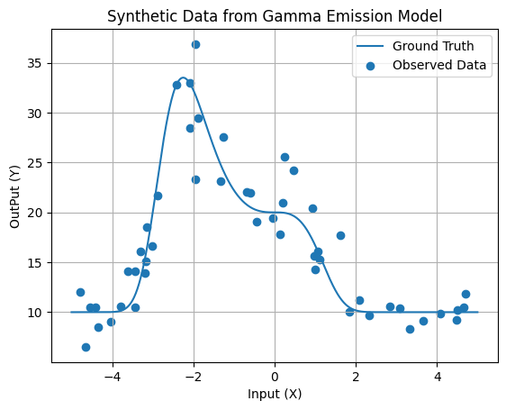
1. Generate Synthetic Data from Gamma Emission Model

We’ll start by generating synthetic data using a custom gamma emission function. This function will simulate the emission of gamma particles, and we’ll add some random noise to the observed data points. This noisy data will serve as our training set.

# Necessary imports
import numpy as np
import matplotlib.pyplot as plt

# Set random seed for reproducibility
np.random.seed(42)

# Define the custom gamma emission function
def groundTruth(x):
    val = 10 * np.exp(-0.1 * (x**4 + 3 * x**3)) + 10
    return val

# Generate synthetic data from the gamma emission model
xData = 10 * np.random.rand(50) - 5
emissionData = groundTruth(xData)
yData = np.random.gamma(25, emissionData / 25)

# Plot the gamma emission model and synthetic data
xFine = np.linspace(-5, 5, 1000)
fFine= groundTruth(xFine)

plt.plot(xFine, fFine, label='Ground Truth')
plt.scatter(xData, yData, label='Observed Data')
plt.xlabel('Input (X)')
plt.ylabel('OutPut (Y)')
plt.title('Synthetic Data from Gamma Emission Model')
plt.legend()
plt.grid(True)
plt.show()

2. Define the Kernel and Posterior

Next, let’s define the squared exponential kernel function and the covariance matrix generator function. These components are essential for Gaussian Process Regression and capturing relationships between data points.

# Define the squared exponential kernel function
def squaredExpKernel(x1, x2, sigma=1.0, lengthScale=1.0):
    val = (sigma**2) * np.exp(-0.5 * ((x2 - x1) / lengthScale)**2)
    return val

# Define the covariance matrix generator function
def covMatGenerator(v1, v2, sigma=1, lengthScale=1):
    K = np.zeros((len(v1), len(v2)))
    for i in range(len(v1)):
        for j in range(len(v2)):
            K[i, j] = squaredExpKernel(v1[i], v2[j], sigma, lengthScale)
    return K

# Generate the covariance matrices for the data and inference points
covSigma = 20
covLength = 1
KDataData = covMatGenerator(xData, xData, covSigma, covLength)
KFineData = covMatGenerator(xFine, xData, covSigma, covLength)
KDataDataInv = np.linalg.inv(KDataData + 0.0001 * np.eye(len(xData)))

# Define the log posterior probability
def logPost(function, data=yData, a=25, covMatInv=KDataDataInv):
    if np.any(function < 0):
        val = -np.inf
    else:
        lhood = -a * np.sum(np.log(function)) + (a - 1) * np.sum(np.log(data)) - np.sum(data / function) * a
        prior = -0.5 * (function.T @ (covMatInv @ function))
        val = lhood + prior
    return val

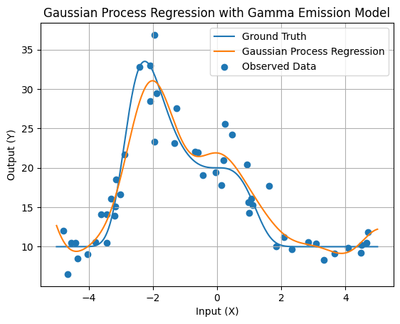
3. Perform Gaussian Process Regression with Gamma Emission Model

Now, let’s perform Gaussian Process Regression using our synthetic data from the gamma emission model. We’ll generate test points, calculate covariance matrices, and predict emission values at these test points. We’ll also visualize the results.

# Initial sample for Metropolis-Hastings
fPred = np.mean(yData) * np.ones(len(xData))
oldProb = logPost(fPred)

# Lists for probability and sample cache
samplesVect = []
pVect = []
samplesVect.append(fPred)
pVect.append(oldProb)

for _ in range(10000):
    proposed = fPred + np.random.multivariate_normal(np.zeros(len(fPred)), KDataData) * 0.05
    newProb = logPost(proposed)

    accRate = newProb - oldProb

    if accRate > np.log(np.random.rand()):
        fPred = proposed
        oldProb = newProb
    samplesVect.append(fPred)
    pVect.append(oldProb)

# Calculate predictions using the covariance matrix and samples
fFinePred = KFineData @ (KDataDataInv @ np.mean(samplesVect, 0))

# Plot the Gaussian Process Regression result with the gamma emission model
plt.plot(xFine, fFine, label='Ground Truth')
plt.plot(xFine, fFinePred, label='Gaussian Process Regression')
plt.scatter(xData, yData, label='Observed Data')
plt.xlabel('Input (X)')
plt.ylabel('Output (Y)')
plt.title('Gaussian Process Regression with Gamma Emission Model')
plt.legend()
plt.grid(True)
plt.show()

In this exploration of Gaussian Processes within the Bayesian paradigm, we’ve traversed the intricate dance between Gaussian Process Regression and the tenets of Bayesian inference. From Bayes’ theorem to non-conjugate likelihoods, we’ve illuminated the threads that weave these concepts into a harmonious fabric of mathematical understanding. As we set our sights on the horizon of computational complexity in Gaussian Process inference, the forthcoming installment promises to illuminate the artistry and science required to navigate these complex waters.