Introduction

For as long as we have been human, we have looked up to the heavens in awe and wonder. We developed the telescope to further explore the cosmos, a tool now employed by both the cutting edges of science and your humble hobbyist. When we gaze through the lens and record our findings, however, our perception of the celestial objects is subtly (or sometimes not-so-subtly) distorted, a product of collaboration between the telescope, the light itself, and the camera employed. Additionally, we find more alterations when there are imperfections in the equipment, resulting in aberrations, and imperfections in the environment, caused by light pollution or air distortion. Here, I guide you through modeling the most direct path from object to final image with the Julia language, leaving discussion of light pollution and aberrations for another time.

Relevant Parameters

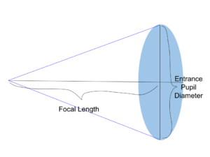
Before we begin to model this process, we must familiarize ourselves with the critical parameters that shape the outcome of our simulations. Firstly, we consider the wavelength of the light we collect. Light waves range from approximately 380 to 750 nanometers within the visible range. Secondly, we consider the telescope, where the numerical aperture is of most importance. This dimensionless metric characterizes the maximum angle at which light can be received, approximated as the half of the ratio of the diameter of the entrance pupil to the focal length.

In addition to the telescope, the camera employed for image acquisition plays a pivotal role in shaping the final result. Several parameters demand our attention, starting with the gain- a measure defining the conversion of individual recorded photons to analog-to-digital units (ADUs). A well-calibrated gain ensures a faithful representation of the detected light, laying the foundation for accurate interpretation and analysis. Another camera parameter we concern ourselves with is the offset, a consistent and deliberate adjustment applied to the entire image to avoid underexposure. By introducing this predetermined offset, we safeguard against the risk of losing valuable information. Furthermore, we must consider the size of each pixel in the camera image. This will inform the scaling for the other parameters. Lastly, we must consider the presence of read noise—an intrinsic characteristic of the camera system. This measure quantifies the random fluctuations that occur during the process of reading the image sensor, influencing the overall image quality. With these quantities acknowledged and obtained, we can proceed with the simulation

Package Statements

We begin our code. For those unfamiliar, Julia is a programming language designed for high performance speed and dynamic programming environments. For this modeling, we we be implementing the following Julia packages:

using Plots
using FFTW
using Distributions
using Random

The Plots package will be used in displaying the images we obtain, which will be modeled as heatmaps. The FFTW package will be used in the deterministic first step of the process, when the object is convoluted with the Point Spread Function. The Distributions and Random packages will be implemented in the probabilistic second step of the process.

Parameter and Object Initialization

At this point, we will initialize our parameters that we discussed two sections prior. The values I give are examples, and the actual values will depend on the light wavelength, telescope, and camera you are modeling.

wavelength = 0.5 #microns, green light
numerical_aperture = 1.2
gain = 2 #ADUs/photon
camera_offset = 100 #ADUs
read_noise = 5 #square root ADUs
pix_size = 4.63 # microns

At this point, I will also calculate the variance of the Point Spread Function (more on that in the next section).

v = (1.22 * wavelength) / (2 * numerical_aperture)

Now, we must initialize the object that we are considering, which, of course, will depend on what we want to model. For this case, we will consider a simple dummy object. Two circles, one brighter and smaller than the other, with a small image size of 100 x 100.

object = zeros(100, 100) #defines pixel grid
for i in 1:size(object,1)
    for j in 1:size(object,2)
        if ((i - 70) ^ 2 + (j - 75) ^ 2 <= 100)
            object[i,j] = 75 #intensity for larger circle
        end
        if ((i - 30) ^ 2 + (j - 15) ^ 2 <= 25)
            object[i,j] = 150 #intensity for smaller circle
        end
    end
end

Of course, to check if the object is what you are expecting, you can display it as a heatmap. This can also be done during all the intermediate steps by swapping “object” with the appropriate variable

heatmap(object, c=:grays, legend=false, yflip=true)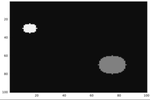

Point Spread Function

The first transformation of our object will be a convolution of it with our Point Spread Function, or PSF. The PSF models how light emitted from a point emitter will spread as it travels through the telescope. The spread of light is most accurately modeled as an Airy Function, but a Normal distribution is a very good approximation, and is sufficient for our purposes. This Normal distribution will be centered at the center of the image, and the variance is proportional to the wavelength and inversely proportional to the numerical aperture, formulated by

$$variance = (1.22 wavelength) / (2 numerical aperture)$$

Similarly to the object, we define the PSF on the grid of pixels.

PSF = zeros(size(object, 1), size(object, 2)) #match size with object
for i in 1:size(PSF, 1)
    for j in 1:size(PSF, 2)
        PSF[i,j] = 1 / sqrt(2 * pi * v) * 
exp(((i - (size(PSF, 1) + 1) / 2) ^ 2 + 
(j - (size(PSF, 2) + 1) / 2) ^ 2) / (-2 * v))
    end
end

Next, we need to convolute the object and PSF. By the Convolution Theorem, the Fourier Transform of our resulting convolution will be the product of the Fourier Transforms of the object and the PSF. To accomplish this, we implement functions from the FFTW package. The Fast Fourier Transform function computes the Fourier Transform for the case of discrete points. Finally, for scaling, the image is multiplied by the area of a pixel.

Fobject = fftshift(fft(object))
FPSF = fftshift(fft(PSF))
noiseless_image = abs.(ifftshift(ifft(Fobject .* FPSF))) .* pix_size ^ 2

Note that we employ the absolute value function in producing the noiseless image. This is to remove aspects that do not make physical sense. Since the Fast Fourier Transform is ultimately an approximation, we may obtain small negative values or imaginary components, which we do not want, as they both are illogical (What does a negative or imaginary intensity mean?) and cause issues in modeling the noise, as we shall see now.

Noise

The first type of noise we model is Shot Noise. This noise comes about from the discrete nature of light. The light is collected at each pixel, with each receiving an integer number of photons. Thus, to represent the discrete nature of photons, the image is subjected to Poisson noise.

shot_image = rand.(Poisson.(noiseless_image))

Afterwards, the image is subjected to camera noise. The way photons are equated to ADUs is a Normal Distribution. The gain is a measure of how many ADUs are counted per photon, so the mean ADU at each pixel will be the gain multiplied by the photon count with the offset added at each point. The standard deviation of the distribution is characterized by our read noise parameter. After the second round of noise, we observe our resulting image.

final_image = rand.(Normal.(gain * shot_image .+ camera_offset, read_noise))
heatmap(final_image, c=:grays, legend=false, yflip=true)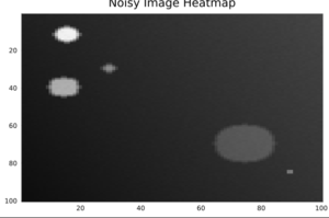

After two types of noise and a convolution, we have concluded our model of how our camera is created from the original celestial object.

Conclusion

With this framework, we simulate how a celestial object will appear in astronomical photos with minimized outside distortion or aberration. This framework can be expanded to model these other sources of image alteration, or altered to model other optical systems, such as in microscopy. Whether you’re a novice to telescoping or a seasoned stargazer, I hope this blog post was insightful and sparked your curiosity in looking up to the stars.