Why do we need Bayesian statistics? Part III – Learning multivariate distributions (tutorial)

• Why do we need Bayesian statistics? Part III – Learning multivariate distributions (tutorial)
  • Introduction
    • The likelihood
    • Prior
    • Posterior
    • Inference
    • Marginal posterior distribution
  • Conclusion

Introduction

In the previous entry of this tutorial series, we studied the lighthouse problem. The goal was to infer (or learn) the position of the lighthouse from observations of where the lighthouse’s light beam hits the floor. A schematic of the problem is presented below.

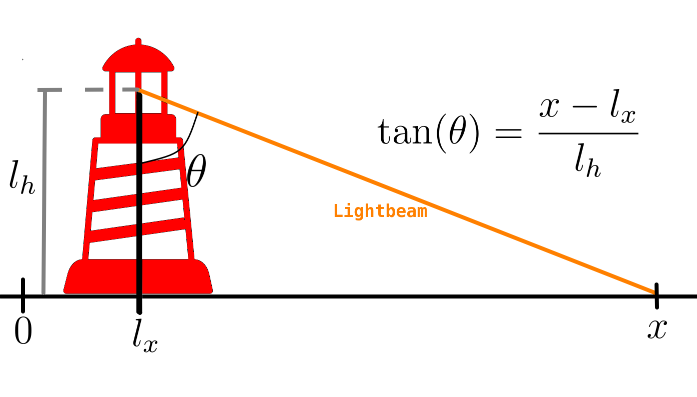
Following what was established on the previous post, let us generate synthetic data for the lighhouse problem. We sample $\theta$ uniformly in $\left( -\frac{\pi}{2}, \frac{\pi}{2} \right)$ and obtain $x$ as

$$tan \theta = \frac{x-l_x}{l_h} \Rightarrow x = l_x + l_h tan \theta \ . \quad \quad \quad (1)$$

import numpy as np
from matplotlib import pyplot as plt
np.random.seed(42)

l_x,l_h = 0,1 #setting ground truth

th = np.pi*(np.random.rand(1024)-1/2) #sample theta
x = l_x +l_h*np.tan(th)

In the previous post we outline how to infer $l_x$, the lighthouse horizontal position, assuming the height, $l_h$ is already known. However, the study of probabilities presented in that post does allow one to infer both $l_x$ and $l_h$ despite the fact that the observation $x$ is univariate.

The likelihood

This is possible by obtaining the conditional probability of a single point $x$ given $l_x$ and $l_h$, as done in the previous blog post, which is given by
$$p(x|l_x,l_h) = \frac{1}{\pi} \frac{l_h}{ (x-l_x)^2 + l_h^2 } \ . \quad \quad \quad (2)$$

For a set of multiple data points $\{x_n\} = \{x_1, x_2,x_3, \ldots , x_N\}$ obtained independently, the conditional probability, or likelihood, of the whole dataset is
$$p(\{x_n\}|l_x,l_h) = \prod_{n=1}^N \left[ \frac{1}{\pi} \frac{l_h}{ (x_n-l_x)^2 + l_h^2 } \right] \ . \quad \quad \quad (3)$$
Which, as in the previous blog post is expressed in terms of the logarithm for numerical stability, yielding
$$\ln p(\{x_n\}|l_x,l_h) = \sum_{n=1}^N \ln \left[ \frac{1}{\pi} \frac{l_h}{ (x_n-l_x)^2 + l_h^2 } \right] . \quad \quad \quad (4)$$
which can be calculated using the following piece of code

def log_like_2d(x,lx,lh):
    LX,LH=np.meshgrid(lx,lh) 
    log_like = np.zeros_like(LX)
    for xi in x:
        log_like += np.log(LH)-np.log(np.pi)-np.log((xi-LX)**2+LH**2)
    return log_like

Here we assume that $l_x$ and $l_h$ were given in a form of an (numpy) array representing all possible values. The choice to represent this way is better explained when we look into the prior.

Prior

In order to infer $l_x$ and $l_h$ we ought to invert the conditional probability using Bayes’ theorem:
$$p(l_x,l_h|\{x_n\}) =\frac{ p(\{x_n\}|l_x,l_h)}{p(\{x_n\})} p(l_x,l_h) \ , \quad \quad \quad (5)$$

with the prior, $p(l_x,l_h)$, chosen in a manner similar to the previous blog post
$$p(l_x,l_h) = \begin{cases} \frac{1}{LH} & \text{for} \ -\frac{L}{2}<l_x<\frac{L}{2} \ \text{and} \ 0< l_h< H \\ 0 & \text{otherwise} \end{cases} \ . \quad \quad \quad (6)$$
Or, in other words, the prior is uniform in $l_x \in (-\frac{L}{2},\frac{L}{2})$ and $l_h \in (0,H)$. For the purposes of later visualization we choose $L = H = 2$, but the results allow for much larger values.

L,H = 2.,2.

First let us generate the arrays for $l_x$ and $l_h$:

lh_arr=np.linspace(0,H,101)+1e-12
lx_arr=np.linspace(-L/2,L/2,101)

this guarantees a good representation of the intervals $l_x \in (-\frac{L}{2},\frac{L}{2})$ and $l_h \in (0,H)$.

Posterior

Going back to the Bayes’ theorem (5), and substituting the prior (6) and likelihood (4) one obtains
$$p(l_x,l_h|\{x_n\}) = \frac{1}{Z’} \ \exp\left[ \sum_{n=1}^N \ln \left[ \frac{1}{\pi} \frac{l_h}{ (x_n-l_x)^2 + l_h^2 } \right] \right] \ . \quad \quad \quad (7)$$
Where $Z’ = LH P(\{x_n\})$, note that $P(\{x_n\})$ in (5) does not depend on $l_x$ or $l_h$. As such, $Z’$ is calculares by ensuring that $\int \mathrm{d} l_h \ \mathrm{d} l_x \ p(l_x,l_h|\{x_n\}) = 1$.
The following block of code gives a function to calculate the posterior (7)

def posterior(x,lx,lh):
    L = log_like_2d(x,lx,lh)
    L -= L.max()

    P = np.exp(L) #unnormalized posterior
    
    dlh,dlx = (lh[1]-lh[0]),(lx[1]-lx[0])
    Z = P.sum()*(dlh*dlx) #normalization factor

    P = P/Z
    return P

Inference

Now that we have the computational tools to calculate the posterior let us visualize how the posterior evolves with the number of datapoints.

Since we are talking about a two dimensional posterior, we present how it evolves with the number of datapoints through an animation (see the complete code in my GitHub repository).

#Removed data block, see notebook on GitHub for full code

Marginal posterior distribution

While in the previous blog post we found the distribution for the lighthouse horizontal position, $l_x$, assuming a known height, $l_h$, here we obtain the distribution for both the $l_h$ and $l_x$, denoted as $p(l_x,l_h|\{x_n\})$. In order to obtain the posterior for only $l_x$ or only for $l_h$ we ought to sum (or integrate) over the probabilities of all possible value of the other parameter, that is:
$$p(l_x|\{x_n\}) = \int \mathrm{d}l_h \ p(l_x,l_h|\{x_n\}) \ , \quad \quad \quad (8a)$$
$$p(l_h|\{x_n\}) = \int \mathrm{d}l_x \ p(l_x,l_h|\{x_n\}) \ . \quad \quad \quad (8b)$$

In probability theory obtaining the probability for one parameter from the integral over the other parameters as above is often referred as marginalization. Moreover, in Bayesian language $p(l_x|\{x_n\})$ and $p(l_h|\{x_n\})$ are the marginalized posteriors while $p(l_x,l_h|\{x_n\})$ is the joint posterior.

It is important to notice that $p(l_x|\{x_n\})$ obtained above is conceptually different for what was done in the previous blog post. While there we considered that $l_h$ was already known here we cover all possible values of $l_h$ based on the posterior, which was learned from data.

In order to give a good visualization of how the marginal posterior for both $l_x$ and $l_h$ evolve with the total number of data points, we show an animation analogous to the previous one but also presenting the marginal posteriors parallel to their respective axis.

#Removed data block, see notebook on GitHub for full code

Here we can see clearly that, as the number of data points increase, the posterior (both the joint and each of the marginalized ones) tightens around the ground truth values.

Conclusion

Here we finish the overarching tutorial on Bayesian statistics. While future posts involving the topic will come, we presented a tutorial where:

1. Bayesian statistics concurs with more naive methods of inference,
2. The system is severely more complex and these naive methods fail, and
3. The present post, where we went further into the previous problems to show how to learn multiple values even when the data available is single-valued.

Although this is the last entry of this tutorial series, more future posts related to the intricacies of probability and statistics in this blog. I hope this was instructive. Stay tuned.